Python profiling

07.04.2020 — python, cloud-shell, profiler, GCS — 2 min read

When you start to program big or start to process bigger data than usual, you can notice slowness sometimes. It could be due to memory used in the laptop at that time. You can retry after shutting down all the application which you have been running parallely. If its still slow, it must because of your code. Easiest way to spot slow section of the code is by setting up timers,

1from time import time, sleep
2step_start = time()
3### Some big process start
4sleep(2.4) 
5### Some big process end
6step_et = time()-step_start
7print("=== {} Total Elapsed time is {} sec\n".format('Sleeping', round(step_et,3) ))

If you want to know how much time entire program takes, you can do something like this,

1$ time python BTD-Analysis1V3.py
2getcwd :  D:\BigData\12. Python\5. BTD\progs
3Length of weekly =  53
4
5real    0m5.441s
6user    0m0.000s
7sys     0m0.062s

Its not always a good strategy to guess or follow the gut-feeling in identifying performance problems, things can surprise you.

If you are looking for more information than the above timers like number of calls, execution time then you should look into Python profilers.

What's Python Profiling ? As per the doc

A profile is a set of statistics that describes how often and for how long various parts of the program executed.

Here we are going to see two profilers,

cProfile
line_profile

# cProfile

This profiler comes in the standard python installation. Easiest way to profile a program is like below,

1python -m cProfile -s cumtime BTD-Analysis1V3.py
2
3# output 
4Sushanth@Sushanth-VAIO MINGW64 /d/BigData/12. Python/5. BTD/progs
5$ python -m cProfile -s cumtime BTD-Analysis1V3.py
6getcwd :  D:\BigData\12. Python\5. BTD\progs
7Length of weekly =  53
8         323489 function calls (315860 primitive calls) in 5.602 seconds
9
10   Ordered by: cumulative time
11
12   ncalls  tottime  percall  cumtime  percall filename:lineno(function)
13    751/1    0.029    0.000    5.606    5.606 {built-in method builtins.exec}
14        1    0.000    0.000    5.606    5.606 BTD-Analysis1V3.py:2(<module>)
15        2    0.000    0.000    3.911    1.955 parsers.py:536(parser_f)
16        2    0.036    0.018    3.911    1.955 parsers.py:403(_read)
17        2    0.002    0.001    3.804    1.902 parsers.py:1137(read)
18...

This could give you huge information, if your program is big.

Fields	Description
ncalls	How many times code was called
tottime	Total time it took(excluding the time of other functions)
percall	How long each call took
cumtime	Total time it took(including the time of other functions)

You can redirect the output to a text file or dump the stats using the -o output filename option in command.

1python -m cProfile -o profile_output BTD-Analysis1V3.py

By using the output file option, you get additional information like,

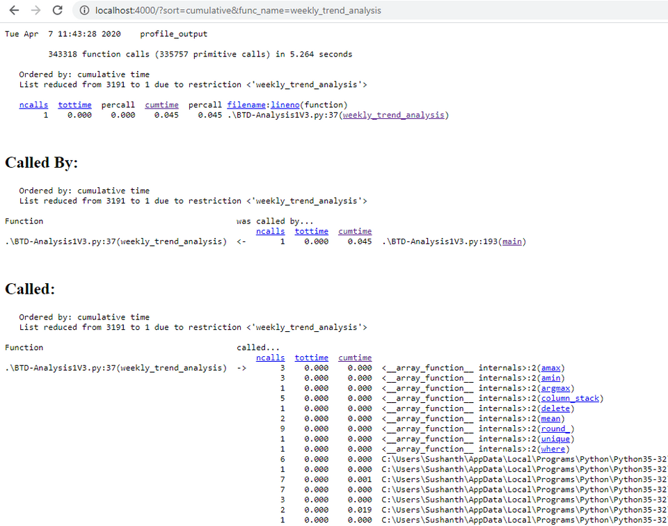
Callers - What function it called
Callees - What function called it

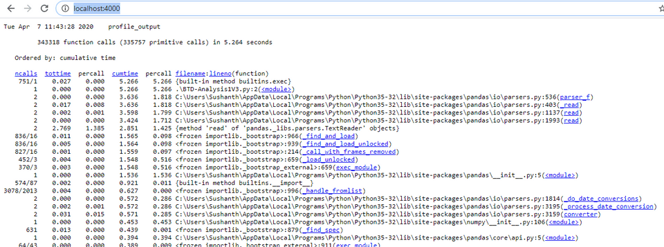
Catch is, this output file is binary. To read this binary file you need to use pstats. All these things sound pretty much tedious. Luckily i found a package called cprofilev which reads this output file and starts a server and in the localhost, where you can see all the profiling information.

Author of the tool : ymichael

Below are the steps,

1# Install
2sudo pip install cprofilev
3
4# Specify the profile output filename
5cprofilev -f profile_output

Now go and check http://localhost:4000/. You will see the stats, you can sort on the fields and click on function name links.

# line_profiler

Problem with this is, i couldn't install line-profiler in Windows 10, failed due to below error and first thing that came to my mind is "i should give up line profiling as it is not getting installed" next thought is "Will this work in Cloud shell".

1Building wheels for collected packages: line-profiler
2  Building wheel for line-profiler (PEP 517) ... error
3  ERROR: Command errored out with exit status 1:
4   command: 'c:\users\sushanth\appdata\local\programs\python\python35-32\python.exe' 'c:\users\sushanth\appdata\local\programs\python\python35-32\lib\site-packages\pip\_vendor\pep517\_in_process.py' build_wheel 'C:\Users\Sushanth\AppData\Local\Temp\tmpktd1yk7q'
5       cwd: C:\Users\Sushanth\AppData\Local\Temp\pip-install-4bud8_nu\line-profiler
6  Complete output (322 lines):
7  Not searching for unused variables given on the command line.
8  -- The C compiler identification is unknown
9  CMake Error at CMakeLists.txt:3 (ENABLE_LANGUAGE):
10    No CMAKE_C_COMPILER could be found.
11
12    Tell CMake where to find the compiler by setting either the environment
13    variable "CC" or the CMake cache entry CMAKE_C_COMPILER to the full path to
14    the compiler, or to the compiler name if it is in the PATH.
15
16
17  -- Configuring incomplete, errors occurred!
18  See also "C:/Users/Sushanth/AppData/Local/Temp/pip-install-4bud8_nu/line-profiler/_cmake_test_compile/build/CMakeFiles/CMakeOutput.log".      
19  See also "C:/Users/Sushanth/AppData/Local/Temp/pip-install-4bud8_nu/line-profiler/_cmake_test_compile/build/CMakeFiles/CMakeError.log".       
20  Not searching for unused variables given on the command line.
21  CMake Error at CMakeLists.txt:2 (PROJECT):
22    Generator
23
24      Visual Studio 15 2017
25
26    could not find any instance of Visual Studio.
27...
28  ERROR: Failed building wheel for line-profiler
29Failed to build line-profiler
30ERROR: Could not build wheels for line-profiler which use PEP 517 and cannot be installed directly

I use Windows 10 machine and to solve the above issue, i took the below steps.

Logged into my google console
Went to Cloud Storage and created a new bucket
Drag and drop files to the bucket ( data files, python file )
Open Cloud Shell and i ran the below commands to set the environment,
```
1gcloud config set project <<project-id>>
```
You can get the project-id by clicking on the top droplist, a small window will open to select the project, where you can see the project-id.

Installed all the required libraries, since its only few

1pip install numpy_indexed
2pip install pandas
3pip install line-profiler

Tested with a small program to see if line profiler works test-lp.py

1from line_profiler import LineProfiler
2import random
3
4def do_stuff(numbers):
5    s = sum(numbers)
6    l = [numbers[i]/43 for i in range(len(numbers))]
7    m = ['hello'+str(numbers[i]) for i in range(len(numbers))]
8
9numbers = [random.randint(1,100) for i in range(1000)]
10lp = LineProfiler()
11lp_wrapper = lp(do_stuff)
12lp_wrapper(numbers)
13lp.print_stats()

Made changes to the source code for line_profiler. Added import for line_profiler,

1from line_profiler import LineProfiler

In my original, i call the function like this,

1df_weekly2 = weekly_trend_analysis(exchange, df_weekly, df_daily)

To profile, i modified the code like this

1lp = LineProfiler()
2lp_wrapper = lp(weekly_trend_analysis)
3lp_wrapper(exchange, df_weekly, df_daily)
4lp.print_stats()

Generates a big output, so its better to save it

1python BTD-Analysis1V3.py > BTD-Prof.txt

When everything is done here, copying outputs & files to cloud storage.

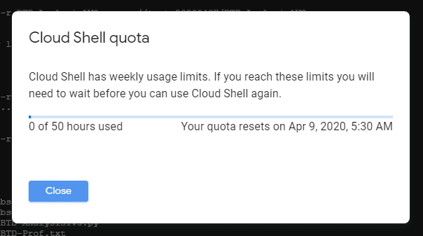
1gsutil -m cp -r BTD-Analysis1V3.py gs://test-20200407/BTD_Analysis1V3-lp.py
2gsutil -m cp -r BTD-Prof.txt gs://test-20200407/BTD-Prof.txt

Cloud shell also has a Quota, watch out for it.

And you are done.

I find Cloud shell handy in doing things like this.

This is how the line-profiler output looks like and i started to work on the code with big Time values.
Details are in here

1('getcwd : ', '/home/bobby_dreamer')
2Timer unit: 1e-06 s
3
4Total time: 0.043637 s
5File: BTD-Analysis1V3.py
6Function: weekly_trend_analysis at line 36
7
8Line #      Hits         Time  Per Hit   % Time  Line Contents
9==============================================================
10    36                                           def weekly_trend_analysis(exchange, df_weekly_all, df_daily):
11    37                                           
12    38         1          3.0      3.0      0.0      if exchange == 'BSE':
13    39         1        963.0    963.0      2.2          ticker = df_daily.iloc[0]['sc_code']
14    40                                               else:
15    41                                                   ticker = df_daily.iloc[0]['symbol']
16    42                                           
17    43         1        201.0    201.0      0.5      arr_yearWeek = df_daily['yearWeek'].to_numpy()
18    44         1        100.0    100.0      0.2      arr_close = df_daily['close'].to_numpy()
19    45         1         87.0     87.0      0.2      arr_prevclose = df_daily['prevclose'].to_numpy()
20    46         1         85.0     85.0      0.2      arr_chng = df_daily['chng'].to_numpy()
21    47         1         83.0     83.0      0.2      arr_chngp = df_daily['chngp'].to_numpy()
22    48         1        108.0    108.0      0.2      arr_ts = df_daily['ts'].to_numpy()
23    49         1         89.0     89.0      0.2      arr_volumes = df_daily['volumes'].to_numpy()
24    50                                           
25    51                                               # Close
26    52         1         41.0     41.0      0.1      arr_concat = np.column_stack((arr_yearWeek, arr_close))
27    53         1        241.0    241.0      0.6      npi_gb = npi.group_by(arr_concat[:, 0]).split(arr_concat[:, 1])
28    54                                           
29    55                                               #a = df_temp[['yearWeek', 'close']].to_numpy()
30    56         1        113.0    113.0      0.3      yearWeek, daysTraded = np.unique(arr_concat[:,0], return_counts=True)
31    57                                               
32    58         1          4.0      4.0      0.0      cmaxs, cmins = [], []
33    59         1          3.0      3.0      0.0      first, last, wChng, wChngp = [], [], [], []
34    60         2         11.0      5.5      0.0      for idx,subarr in enumerate(npi_gb):
35    61         1         32.0     32.0      0.1          cmaxs.append( np.amax(subarr) )
36    62         1         17.0     17.0      0.0          cmins.append( np.amin(subarr) )
37    63         1          2.0      2.0      0.0          first.append(subarr[0])
38    64         1          2.0      2.0      0.0          last.append(subarr[-1])
39    65         1          3.0      3.0      0.0          wChng.append( subarr[-1] - subarr[0] )
40    66         1          6.0      6.0      0.0          wChngp.append( ( (subarr[-1] / subarr[0]) * 100) - 100 )
41    67                                           
42    68                                               #npi_gb.clear()
43    69         1          4.0      4.0      0.0      arr_concat = np.empty((100,100))
44    70                                           
45    71                                               # Chng
46    72         1         21.0     21.0      0.0      arr_concat = np.column_stack((arr_yearWeek, arr_chng))
47    73         1        109.0    109.0      0.2      npi_gb = npi.group_by(arr_concat[:, 0]).split(arr_concat[:, 1])
48    74                                           
49    75         1          2.0      2.0      0.0      HSDL, HSDG = [], []
50    76         2          7.0      3.5      0.0      for idx,subarr in enumerate(npi_gb):
51    77         1         12.0     12.0      0.0          HSDL.append( np.amin(subarr) )
52    78         1          9.0      9.0      0.0          HSDG.append( np.amax(subarr) )
53    79                                           
54    80                                               #npi_gb.clear()
55    81         1          3.0      3.0      0.0      arr_concat = np.empty((100,100))
56    82                                           
57    83                                               # Chngp
58    84         1         15.0     15.0      0.0      arr_concat = np.column_stack((arr_yearWeek, arr_chngp))
59    85         1         86.0     86.0      0.2      npi_gb = npi.group_by(arr_concat[:, 0]).split(arr_concat[:, 1])
60    86                                           
61    87         1          1.0      1.0      0.0      HSDLp, HSDGp = [], []
62    88         2          7.0      3.5      0.0      for idx,subarr in enumerate(npi_gb):
63    89         1         11.0     11.0      0.0          HSDLp.append( np.amin(subarr) )
64    90         1          9.0      9.0      0.0          HSDGp.append( np.amax(subarr) )
65    91                                           
66    92                                               #npi_gb.clear()
67    93         1          3.0      3.0      0.0      arr_concat = np.empty((100,100))
68    94                                           
69    95                                               # Last Traded Date of the Week
70    96         1       3111.0   3111.0      7.1      i = df_daily[['yearWeek', 'ts']].to_numpy()
71    97         1        128.0    128.0      0.3      j = npi.group_by(i[:, 0]).split(i[:, 1])
72    98                                           
73    99         1          2.0      2.0      0.0      lastTrdDoW = []
74   100         2          9.0      4.5      0.0      for idx,subarr in enumerate(j):
75   101         1          2.0      2.0      0.0          lastTrdDoW.append( subarr[-1] )
76   102                                           
77   103         1          4.0      4.0      0.0      i = np.empty((100,100))
78   104                                               #j.clear()
79   105                                           
80   106                                               # Times inreased
81   107         1         11.0     11.0      0.0      TI = np.where(arr_close > arr_prevclose, 1, 0)
82   108                                           
83   109                                               # Below npi_gb_yearWeekTI is used in volumes section
84   110         1         19.0     19.0      0.0      arr_concat = np.column_stack((arr_yearWeek, TI))
85   111         1        111.0    111.0      0.3      npi_gb_yearWeekTI = npi.group_by(arr_concat[:, 0]).split(arr_concat[:, 1])
86   112                                           
87   113         1         73.0     73.0      0.2      tempArr, TI = npi.group_by(arr_yearWeek).sum(TI)
88   114                                           
89   115                                               # Volume ( dependent on above section value t_group , thats the reason to move from top to here)
90   116         1         39.0     39.0      0.1      arr_concat = np.column_stack((arr_yearWeek, arr_volumes))
91   117         1         94.0     94.0      0.2      npi_gb = npi.group_by(arr_concat[:, 0]).split(arr_concat[:, 1])
92   118                                           
93   119         1          2.0      2.0      0.0      vmaxs, vavgs, volAvgWOhv, HVdAV, CPveoHVD, lastDVotWk, lastDVdAV = [], [], [], [], [], [], []
94   120         2          8.0      4.0      0.0      for idx,subarr in enumerate(npi_gb):
95   121         1         53.0     53.0      0.1          vavgs.append( np.mean(subarr) )
96   122         1          2.0      2.0      0.0          ldvotWk = subarr[-1]
97   123         1          2.0      2.0      0.0          lastDVotWk.append(ldvotWk)
98   124                                           
99   125                                                   #print(idx, 'O - ',subarr, np.argmax(subarr), ', average : ',np.mean(subarr))
100   126         1         13.0     13.0      0.0          ixDel = np.argmax(subarr)
101   127         1          2.0      2.0      0.0          hV = subarr[ixDel]
102   128         1          2.0      2.0      0.0          vmaxs.append( hV )
103   129                                           
104   130         1          1.0      1.0      0.0          if(len(subarr)>1):
105   131         1         53.0     53.0      0.1              subarr = np.delete(subarr, ixDel)
106   132         1         29.0     29.0      0.1              vawoHV = np.mean(subarr)
107   133                                                   else:
108   134                                                       vawoHV = np.mean(subarr)
109   135         1          2.0      2.0      0.0          volAvgWOhv.append( vawoHV )
110   136         1         12.0     12.0      0.0          HVdAV.append(hV / vawoHV)
111   137         1          3.0      3.0      0.0          CPveoHVD.append( npi_gb_yearWeekTI[idx][ixDel] )
112   138         1          6.0      6.0      0.0          lastDVdAV.append(ldvotWk / vawoHV)    
113   139                                           
114   140                                               #npi_gb.clear()
115   141         1          3.0      3.0      0.0      arr_concat = np.empty((100,100))
116   142                                           
117   143                                               # Preparing the dataframe
118   144                                               # yearWeek and occurances 
119   145                                               #yearWeek, daysTraded = np.unique(a[:,0], return_counts=True)
120   146         1          5.0      5.0      0.0      yearWeek = yearWeek.astype(int)
121   147         1         44.0     44.0      0.1      HSDL = np.round(HSDL,2)
122   148         1         21.0     21.0      0.0      HSDG = np.round(HSDG,2)
123   149         1         18.0     18.0      0.0      HSDLp = np.round(HSDLp,2)
124   150         1         18.0     18.0      0.0      HSDGp = np.round(HSDGp,2)
125   151                                           
126   152         1         17.0     17.0      0.0      first = np.round(first,2)
127   153         1         17.0     17.0      0.0      last = np.round(last,2)
128   154         1         17.0     17.0      0.0      wChng = np.round(wChng,2)
129   155         1         16.0     16.0      0.0      wChngp = np.round(wChngp,2)
130   156                                           
131   157         1          5.0      5.0      0.0      vavgs = np.array(vavgs).astype(int)
132   158         1          3.0      3.0      0.0      volAvgWOhv = np.array(volAvgWOhv).astype(int)
133   159         1         17.0     17.0      0.0      HVdAV = np.round(HVdAV,2)
134   160                                           
135   161         1          3.0      3.0      0.0      dict_temp = {'yearWeek': yearWeek, 'closeH': cmaxs, 'closeL': cmins, 'volHigh':vmaxs, 'volAvg':vavgs, 'daysTraded':daysTraded
136   162         1          2.0      2.0      0.0                  ,'HSDL':HSDL, 'HSDG':HSDG, 'HSDLp':HSDLp, 'HSDGp':HSDGp, 'first':first, 'last':last, 'wChng':wChng, 'wChngp':wChngp
137   163         1          2.0      2.0      0.0                  ,'lastTrdDoW':lastTrdDoW, 'TI':TI, 'volAvgWOhv':volAvgWOhv, 'HVdAV':HVdAV, 'CPveoHVD':CPveoHVD
138   164         1          2.0      2.0      0.0                  ,'lastDVotWk':lastDVotWk, 'lastDVdAV':lastDVdAV}
139   165         1       3677.0   3677.0      8.4      df_weekly = pd.DataFrame(data=dict_temp)
140   166                                           
141   167         1       1102.0   1102.0      2.5      df_weekly['sc_code'] = ticker
142   168                                           
143   169         1          3.0      3.0      0.0      cols = ['sc_code', 'yearWeek', 'lastTrdDoW', 'daysTraded', 'closeL', 'closeH', 'volAvg', 'volHigh'
144   170         1          1.0      1.0      0.0               , 'HSDL', 'HSDG', 'HSDLp', 'HSDGp', 'first', 'last', 'wChng', 'wChngp', 'TI', 'volAvgWOhv', 'HVdAV'
145   171         1          2.0      2.0      0.0               , 'CPveoHVD', 'lastDVotWk', 'lastDVdAV']
146   172                                           
147   173         1       2816.0   2816.0      6.5      df_weekly = df_weekly[cols].copy()
148   174                                                   
149   175                                               # df_weekly_all will be 0, when its a new company or its a FTA(First Time Analysis)
150   176         1         13.0     13.0      0.0      if df_weekly_all.shape[0] == 0:
151   177         1      20473.0  20473.0     46.9          df_weekly_all = pd.DataFrame(columns=list(df_weekly.columns))       
152   178                                                   
153   179                                               # Removing all yearWeek in df_weekly2 from df_weekly
154   180         1        321.0    321.0      0.7      a = set(df_weekly_all['yearWeek'])
155   181         1        190.0    190.0      0.4      b = set(df_weekly['yearWeek'])
156   182         1          5.0      5.0      0.0      c = list(a.difference(b))
157   183                                               #print('df_weekly_all={}, df_weekly={}, difference={}'.format(len(a), len(b), len(c)) )
158   184         1       1538.0   1538.0      3.5      df_weekly_all = df_weekly_all[df_weekly_all.yearWeek.isin(c)].copy()
159   185                                           
160   186                                               # Append the latest week data to df_weekly
161   187         1       6998.0   6998.0     16.0      df_weekly_all = pd.concat([df_weekly_all, df_weekly], sort=False)
162   188                                               #print('After concat : df_weekly_all={}'.format(df_weekly_all.shape[0]))    
163   189                                                   
164   190         1          2.0      2.0      0.0      return df_weekly_all