Hello BigQuery
BigQuery is a fully-managed enterprise data warehouse that helps you manage and analyze your data with built-in features like machine learning, geospatial analysis, and business intelligence. BigQuery's serverless architecture with zero infrastructure management lets you query terabytes in seconds and petabytes in minutes and data is stored in columnar format.
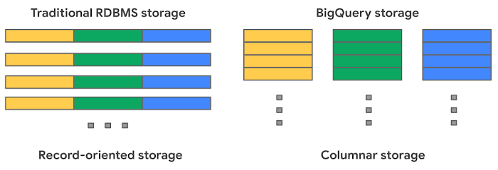
Traditional relational databases, like Db2, Oracle and MySQL, store data in record-oriented storage. This makes them great for transactional updates and OLTP use cases because they only need to open up a single row to read or write data. BigQuery uses columnar storage where each column is stored in a separate file block. This makes BigQuery an ideal solution for OLAP (Online Analytical Processing) use cases.
Contents
Things to know before starting
BigQuery Concepts
BigQuery Objects
Things to know before starting
Limits
NOTE: There is a page dedicated to Limits and Quotas. Here are few which i need to remember.
- Your project can make up to 1,500 table operations per table per day, whether the operation appends data to the table or truncates the table. This limit includes the combined total of all load jobs, copy jobs, and query jobs that append to or overwrite a destination table or that use a DML DELETE, INSERT, MERGE, TRUNCATE TABLE, or UPDATE statement to write data to a table.
- BigQuery runs up to two concurrent mutating DML statements (UPDATE, DELETE, and MERGE) for each table. Additional mutating DML statements for a table are queued.
- A table can have up to 20 mutating DML statements in the queue waiting to run. If you submit additional mutating DML statements for the table, then those statements fail.
- The total size for all of your CSV, JSON, Avro, Parquet, and ORC input files can be up to 15 TB.
- CSV cells/ row can be up to 100 MB in size.
- Your project can run an unlimited number of queries per day.
- A source dataset can have up to 20,000 tables.
- Each partitioned table can have up to 4,000 partitions.
- A table can have up to 10,000 columns.
- A Standard SQL query can have up to 10,000 parameters.
- Each external table can have up to 10,000 source URIs.
Before starting to code
- Doesn't have unique constraints or primary keys
- No Indexes(so no accesspaths, so everything is a scan)
- Supports DML Statements
- Case-sensitive in string comparison and object names refered in FROM clauses but column names are case-sensitive.
- Uses 3-part names to refer to tables {project-id}.{bq-dataset}.{table-name}
- When you write query results to a permanent table, the tables you're querying must be in the same location as the dataset that contains the destination table.
- Use BigQueries
bq cpcommand to copy tables with in the same project or to a different project with 0 cost.
Basic Pricing Information
- With on-demand pricing, BigQuery charges for the number of bytes processed
- The first 1 TB of query data processed per month is free and then its $6.00 per TB
- You're charged according to the total data processed in the columns you select, and the total data per column is calculated based on the types of data in the column. In simple words, you are charged for the sum of bytes in all the columns referenced from the tables scanned by the query, plus the sum of bytes for all columns in the updated table at the time the UPDATE/DELETE starts.
- First 10 GB of storage per month is free and then $0.020 per GB
BigQuery Concepts
Architecture
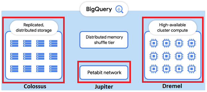
- Colossus : BigQuery leverages the columnar storage format and compression algorithm to store data in Colossus, optimized for reading large amounts of structured data.
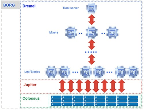
- Dremel : Its the query engine turns SQL queries into execution trees. The leaves of the tree are called slots and do the heavy lifting of reading data from storage and any necessary computation. The branches of the tree are ‘mixers’, which perform the aggregation. To increase performance, each slots work independently from one another. They use Distributed Memory Shuffle to store intermediate results. Each shuffled row can be consumed by workers as soon as it’s created by the producers.
- Jupiter : All these data movement is handled by this super-fast network.
BigQuery is orchestrated via Borg, Google’s precursor to Kubernetes.
Some BigQuery Terminologies
Everything is a job is bigquery, when you query, create, load, export/copy everything creates and submits a batch job in the background and gets you the result. Application may show this as interactive but its actually not. Only a few things that are not managed by a job is listing resources or getting metadata.
BigQuery determines the location to run the job based on the datasets referenced in the request, since the job itself must be run in the same region where the data is stored.
A slot is a unit of computational capacity. It’s basically a worker, made up of CPU, RAM and Network. Since BigQuery likes to divide-and-conquer work - running parts of each task in parallel - more slots usually means that the query will run faster. Number of slots are determined by on-demand pricing and flat-rate pricing
How BigQuery query processing work ?
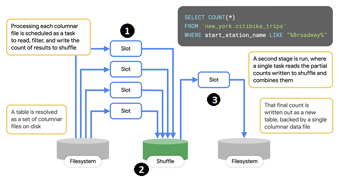
- In the first stage, set of slots will read distributed storage to read in the table. Input table is made up of set of input file blocks. For each input block, a slot is needed to process the file, read and filter down the rows.
- Each worker(in slot) will write one record into shuffle that contains the partial count for the input file.
- Second stage reads from the shuffe records as its input and then sums them together. It then writes the output file into a single file, which because accessible as the results of the query.
Two ways of improving query performance
Partitioning - Table is divided into multiple files/datasets/segments called partitions. Queries that contain filters on the partitioning column can dramatically reduce the overall data scanned. BigQuery supports 3 types of partitions
- Ingestion time partitioned tables: daily partitions reflecting the time the data was ingested into BigQuery.
- Time-unit column partitioned tables: BigQuery routes data to the appropriate partition based on date value in the partitioning column.
- INTEGER range partitioned tables: Partitioned based on an integer column that can be bucketed.
Partitioning is better with column having low cardinality and its recommended that partitions are greater than 1GB.
Clustering - Data can be automatically sorted based on the contents of one or more columns (up to 4, that you specify). Usually high cardinality and non-temporal columns are preferred for clustering. BigQuery performs free, automatic re-clustering in the background.
BigQuery sorts the data in a clustered table based on the values in the clustering columns and organizes them into blocks.
When you run a query against a clustered table, and the query includes a filter on the clustered columns, BigQuery uses the filter expression and the block metadata to prune the blocks scanned by the query. This allows BigQuery to scan only the relevant blocks.
When a block is pruned, it is not scanned. Only the scanned blocks are used to calculate the bytes of data processed by the query. The number of bytes processed by a query against a clustered table equals the sum of the bytes read in each column referenced by the query in the scanned blocks.
BigQuery Objects
Data types
This matters, you are going to be charged for everything that is going to be returned from a SELECT clause and for storage as well.
| Data types | length |
|---|---|
| INT64/INTEGER | 8 bytes (-9,223,372,036,854,775,808 to 9,223,372,036,854,775,807) |
| FLOAT64/FLOAT | 8 bytes |
| NUMERIC | 16 bytes (Precision: 38, Scale: 9) |
| BIGNUMERIC | 32 bytes |
| BOOL/BOOLEAN | 1 byte |
| STRING | 2 bytes + the UTF-8 encoded string size |
| BYTES | 2 bytes + the number of bytes in the value |
| DATE | 8 bytes (0001-01-01) |
| DATETIME | 8 bytes (0001-01-01 00:00:00) |
| TIME | 8 bytes (23:59:59.99999) |
| TIMESTAMP | 8 bytes (9999-12-31 23:59:59.999999 UTC, eg:- 2014-09-27 12:30:00.45-8:00) |
| INTERVAL | 16 bytes |
| STRUCT/RECORD | 0 bytes + the size of the contained fields |
| GEOGRAPHY | 16 bytes + 24 bytes * the number of vertices in the geography type. To verify the number of vertices, use the ST_NumPoints function. |
Null values for any data type are calculated as 0 bytes.
BigQuery Tables
Primarily there are two types of tables
- Permanent tables - Regular tables backed persistent storage
- Temporary tables - BigQuery writes all query results to a table. There are no storage costs for temporary. They are of two types of temporary tables
Created Temporary tables
They can be only be created/refered in a script. These temporary tables exist at the session level, they are created in a special dataset. They are automatically deleted after 24 hours. In the session, to refer TEMP table, you don't need to specify 3-part qualifier like project or dataset qualifier in the table name but when the session completes, you cannot refer it by the same name as a random name is given to it.
1Begin23CREATE TEMP TABLE test_temp as4select *5from `btd_in3.calender`6order by ts desc7limit 5;89End ;
Some important things to know about temporary tables,
Query results are not cached,
- If any of the referenced tables or logical views have changed since the results were previously cached.
- If you are querying multiple tables using a wildcard
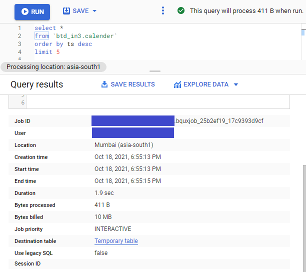
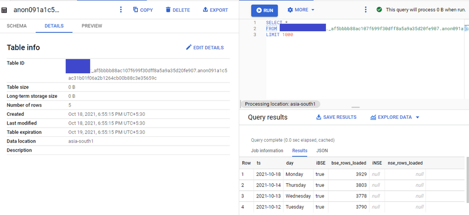
If you have executed a query in BQ console, you can find what temporary it had used by this technique.
At the bottom of the screen, there would be QUERY HISTORY, find the query you had executed. Click it.
Click the Destination table link
It will show you the table, you can look at the SCHEMA, DETAILS, PREVIEW and you can query it if you want.
If you need temporary tables that needs to be refered later by name or it needs to persist more than 24Hours. Create a permanent table with expiration.
1CREATE TABLE `test_public_data.expiry_table`2OPTIONS(3 expiration_timestamp=TIMESTAMP_ADD(CURRENT_TIMESTAMP(), INTERVAL 2 DAY)4) AS5SELECT corpus, COUNT(*) c6FROM `bigquery-public-data.samples.shakespeare`7GROUP BY corpus
External tables -- Data can be queried from external datasources like Cloud Storage, BigTable, Google Drive and CloudSQL.
This example uses schema auto-detection feature. Option available to mention schema details as well.
1CREATE EXTERNAL TABLE `<<project-name>>.test_public_data.test_external_gcs` OPTIONS (2 format = 'CSV',3 uris = ['gs://<<bucket-name>>/bse/bhavcopy_csv/*.CSV']4);Below are the table details,
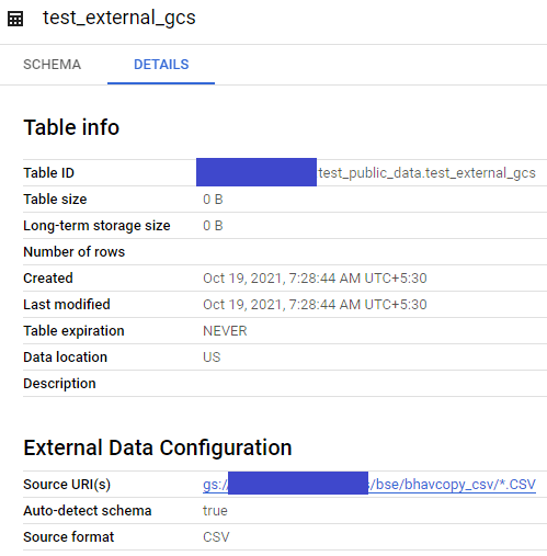
You can query like just another BQ table
1SELECT *2FROM `<<project-name>>.test_public_data.test_external_gcs`3limit 10;Note: Data source and BQ Dataset have to be in same location.